Image Classification is another interesting topic of machine learning. It involves teaching a machine to see and interpret the content of visual data, much like we previously taught models to understand the sentiment of text.
To tackle this visual challenge, we need a new kind of architecture. The star of this show is the Convolutional Neural Network (CNN), an architecture specifically designed to understand and interpret visual information. Unlike our previous text-based models, it excels at recognizing patterns and hierarchical features directly from pixel data.
Our humble goal here is to build a simple CNN, understand its fundamental components, and train it to distinguish between ten different categories of everyday objects using a relatively small dataset.
Data Preparation
For this task, we are going to use a CIFAR-10 dataset, which is conveniently available through Keras. It consists of 60,000 images in 10 classes, with 6,000 images per class.
from datasets import load_dataset
import numpy as np

train, test = load_dataset('uoft-cs/cifar10', split=['train', 'test'])
class_names = train.features['label'].names

x_train = np.array(train['img'])
y_train = np.array(train['label'])
x_test = np.array(test['img'])
y_test = np.array(test['label'])
Output
Let’s visualize a few training images to get a feel for the data.
import matplotlib.pyplot as plt
plt.figure(figsize=[10, 10])

for i in range(25):
    plt.subplot(5, 5, i + 1)
    plt.xticks([])
    plt.yticks([])
    plt.grid(False)
    plt.imshow(x_train[i])
    plt.xlabel(class_names[y_train[i]])

plt.show()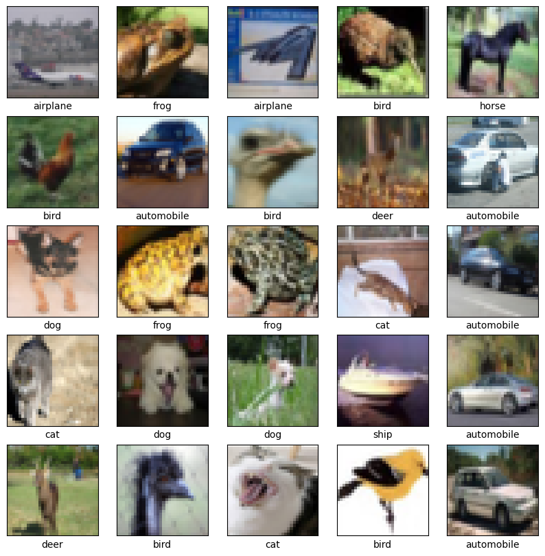
From a technical perspective, each sample (image) is a 32x32 grid of pixels, each encoded using three RGB channels (with their values ranging from 0 to 255). It may be an issue because features with larger numerical values may disproportionately influence the model’s weight updates. Therefore, normalizing them to a smaller range (commonly 0 to 1) would be a good idea.
import numpy as np
x_train = np.array([np.array(x) for x in x_train]).astype('float32') / 255.0
x_test = np.array([np.array(x) for x in x_test]).astype('float32') / 255.0
Building and Training the Model
Now, let’s construct our CNN.
That type of neural network is particularly well-suited for image data because it uses specialized layers to automatically and adaptively learn spatial hierarchies of features – from edges and textures in earlier layers to more complex patterns and object parts in deeper layers.
Our architecture will consist of two sequential sub-models:
Feature Learning: The eyes of the network. This part is responsible for taking the raw pixel data from the image and gradually extracting increasingly complex and abstract visual patterns. Much like how your own visual cortex detects edges, textures, and simple shapes before your brain starts to assemble them into recognizable objects. This is achieved by flowing data through multiple similar stages:
Convolutional Layer: This is the core feature detector. It applies a set of learnable filters (kernels) to the input image. Each filter slides across the image, performing a convolution operation to detect specific features like edges, corners, or textures. Early layers might detect simple lines, while deeper ones combine those into more complex shapes like corners or curves.
Max Pooling Layer: After a convolutional layer has identified a bunch of features, max pooling helps to generalize and condense this information. It looks at small windows of the feature map and picks out the strongest response (the max value). This makes the learned features more robust to variations and greatly reduces computational complexity.
Classification: The brain of the network. Once the feature learning part has extracted a rich set of abstract features from the image, this sub-model takes those high-level features and makes a decision about what object the image contains. Conceptually, it’s very close to our Multilayer Perceptron attempt, but this time it classifies visual clues instead of words.
from tensorflow.keras.utils import set_random_seed
from tensorflow.keras import layers, Sequential
set_random_seed(0)

feature_learning = Sequential(name='feature_learning', layers=[
    layers.Input(shape=x_train.shape[1:]),
    layers.Conv2D(32, (3, 3), activation='relu', padding='same'),
    layers.MaxPooling2D((2, 2)),
    layers.Conv2D(64, (3, 3), activation='relu', padding='same'),
    layers.MaxPooling2D((2, 2)),
    layers.Conv2D(128, (3, 3), activation='relu', padding='same'),
    layers.MaxPooling2D((2, 2)),
])

classification = Sequential(name='classification', layers=[
    layers.Flatten(),
    layers.Dense(128, activation='relu'),
    layers.Dropout(0.5),
    layers.Dense(len(class_names), activation='softmax'),
])

model = Sequential([
    feature_learning,
    classification,
])

display(model.summary(expand_nested=True))Let’s train our model now. We may revert back to CPU usage - our model is yet relatively small.
from tensorflow import device
with device('/CPU'):
    model.compile(optimizer='adam', loss='sparse_categorical_crossentropy', metrics=['accuracy'])
    history = model.fit(x_train, y_train, epochs=25, batch_size=64, validation_split=0.2)
Output
Epoch 1/25
625/625 ━━━━━━━━━━━━━━━━━━━━ 18s 28ms/step - accuracy: 0.2833 - loss: 1.9243 - val_accuracy: 0.4893 - val_loss: 1.3676
Epoch 2/25
625/625 ━━━━━━━━━━━━━━━━━━━━ 17s 28ms/step - accuracy: 0.4947 - loss: 1.4071 - val_accuracy: 0.5787 - val_loss: 1.1928
Epoch 3/25
625/625 ━━━━━━━━━━━━━━━━━━━━ 20s 32ms/step - accuracy: 0.5790 - loss: 1.1937 - val_accuracy: 0.6389 - val_loss: 1.0099
Epoch 4/25
625/625 ━━━━━━━━━━━━━━━━━━━━ 21s 33ms/step - accuracy: 0.6236 - loss: 1.0644 - val_accuracy: 0.6721 - val_loss: 0.9262
Epoch 5/25
625/625 ━━━━━━━━━━━━━━━━━━━━ 21s 33ms/step - accuracy: 0.6587 - loss: 0.9777 - val_accuracy: 0.6783 - val_loss: 0.9039
Epoch 6/25
625/625 ━━━━━━━━━━━━━━━━━━━━ 20s 32ms/step - accuracy: 0.6896 - loss: 0.8862 - val_accuracy: 0.7021 - val_loss: 0.8382
Epoch 7/25
625/625 ━━━━━━━━━━━━━━━━━━━━ 19s 30ms/step - accuracy: 0.7100 - loss: 0.8196 - val_accuracy: 0.6927 - val_loss: 0.8815
Epoch 8/25
625/625 ━━━━━━━━━━━━━━━━━━━━ 19s 31ms/step - accuracy: 0.7312 - loss: 0.7711 - val_accuracy: 0.7164 - val_loss: 0.8269
Epoch 9/25
625/625 ━━━━━━━━━━━━━━━━━━━━ 20s 31ms/step - accuracy: 0.7452 - loss: 0.7205 - val_accuracy: 0.7243 - val_loss: 0.7961
Epoch 10/25
625/625 ━━━━━━━━━━━━━━━━━━━━ 19s 31ms/step - accuracy: 0.7586 - loss: 0.6733 - val_accuracy: 0.7127 - val_loss: 0.8475
Epoch 11/25
625/625 ━━━━━━━━━━━━━━━━━━━━ 21s 34ms/step - accuracy: 0.7738 - loss: 0.6388 - val_accuracy: 0.7304 - val_loss: 0.8007
Epoch 12/25
625/625 ━━━━━━━━━━━━━━━━━━━━ 23s 36ms/step - accuracy: 0.7858 - loss: 0.6018 - val_accuracy: 0.7182 - val_loss: 0.8595
Epoch 13/25
625/625 ━━━━━━━━━━━━━━━━━━━━ 19s 31ms/step - accuracy: 0.7966 - loss: 0.5627 - val_accuracy: 0.7287 - val_loss: 0.8525
Epoch 14/25
625/625 ━━━━━━━━━━━━━━━━━━━━ 18s 29ms/step - accuracy: 0.8082 - loss: 0.5278 - val_accuracy: 0.7127 - val_loss: 0.9415
Epoch 15/25
625/625 ━━━━━━━━━━━━━━━━━━━━ 19s 30ms/step - accuracy: 0.8107 - loss: 0.5158 - val_accuracy: 0.7371 - val_loss: 0.8592
Epoch 16/25
625/625 ━━━━━━━━━━━━━━━━━━━━ 18s 30ms/step - accuracy: 0.8235 - loss: 0.4914 - val_accuracy: 0.7354 - val_loss: 0.8846
Epoch 17/25
625/625 ━━━━━━━━━━━━━━━━━━━━ 18s 29ms/step - accuracy: 0.8256 - loss: 0.4690 - val_accuracy: 0.7255 - val_loss: 0.9586
Epoch 18/25
625/625 ━━━━━━━━━━━━━━━━━━━━ 18s 29ms/step - accuracy: 0.8377 - loss: 0.4482 - val_accuracy: 0.7328 - val_loss: 0.9210
Epoch 19/25
625/625 ━━━━━━━━━━━━━━━━━━━━ 18s 28ms/step - accuracy: 0.8391 - loss: 0.4375 - val_accuracy: 0.7347 - val_loss: 0.9172
Epoch 20/25
625/625 ━━━━━━━━━━━━━━━━━━━━ 18s 28ms/step - accuracy: 0.8433 - loss: 0.4285 - val_accuracy: 0.7340 - val_loss: 0.9364
Epoch 21/25
625/625 ━━━━━━━━━━━━━━━━━━━━ 19s 31ms/step - accuracy: 0.8548 - loss: 0.3911 - val_accuracy: 0.7267 - val_loss: 0.9894
Epoch 22/25
625/625 ━━━━━━━━━━━━━━━━━━━━ 18s 29ms/step - accuracy: 0.8577 - loss: 0.3844 - val_accuracy: 0.7335 - val_loss: 1.0462
Epoch 23/25
625/625 ━━━━━━━━━━━━━━━━━━━━ 19s 30ms/step - accuracy: 0.8647 - loss: 0.3655 - val_accuracy: 0.7417 - val_loss: 1.0008
Epoch 24/25
625/625 ━━━━━━━━━━━━━━━━━━━━ 19s 30ms/step - accuracy: 0.8699 - loss: 0.3565 - val_accuracy: 0.7325 - val_loss: 1.0478
Epoch 25/25
625/625 ━━━━━━━━━━━━━━━━━━━━ 18s 28ms/step - accuracy: 0.8689 - loss: 0.3537 - val_accuracy: 0.7361 - val_loss: 1.0778
import matplotlib.pyplot as plt
plt.figure(figsize=(4.5, 3))
plt.plot(history.history['accuracy'], label='train')
plt.plot(history.history['val_accuracy'], label='validation')
plt.ylabel('accuracy')
plt.xlabel('epoch')
plt.legend(loc='lower right')
plt.show()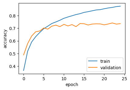
Result
from sklearn.metrics import classification_report
with device('/CPU'):
    y_pred_values = model.predict(x_test, verbose=False)
    y_pred_labels = np.argmax(y_pred_values, axis=1)
    print(classification_report(y_test, y_pred_labels, target_names=class_names))
precision recall f1-score support
airplane 0.76 0.80 0.78 1000
automobile 0.88 0.81 0.85 1000
bird 0.66 0.59 0.62 1000
cat 0.54 0.53 0.54 1000
deer 0.66 0.73 0.70 1000
dog 0.65 0.62 0.64 1000
frog 0.78 0.81 0.80 1000
horse 0.76 0.80 0.78 1000
ship 0.86 0.84 0.85 1000
truck 0.81 0.82 0.81 1000
accuracy 0.74 10000
macro avg 0.74 0.74 0.74 10000
weighted avg 0.74 0.74 0.74 10000
from sklearn.metrics import ConfusionMatrixDisplay
import matplotlib.pyplot as plt
_, ax = plt.subplots(1, 1, figsize=(3.5, 3.5))
ConfusionMatrixDisplay.from_predictions(
    y_test,
    y_pred_labels,
    display_labels=class_names,
    normalize='pred',
    xticks_rotation='vertical',
    include_values=False,
    ax=ax
)
<sklearn.metrics._plot.confusion_matrix.ConfusionMatrixDisplay at 0x173527af0>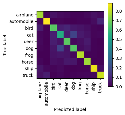
Conclusion
With a respectable 74% accuracy on the CIFAR-10 test set, our relatively straightforward CNN has demonstrated its ability to learn meaningful visual features and classify images, even without extensive tuning or advanced architectures.
This experiment demonstrates how convolutional and pooling layers work together to extract hierarchical patterns, and how a dense classifier can then make sense of these learned features.
Looking at the training history, we can observe the training accuracy steadily increasing. However, the validation accuracy appears to plateau or slightly decrease in later epochs, suggesting that the model is starting to overfit the training data. This suggests a clear need for data augmentation and regularization (batch normalization, more dropouts) to combat this and potentially improve generalization.