In our previous attempt at image classification, we built a pretty decent convolutional neural network and achieved a respectable 74% accuracy on the CIFAR-10 dataset. However, we also observed a clear sign of overfitting - while training accuracy climbed, validation accuracy began to plateau and even dip.
In this notebook, we will try to mitigate this issue by using multiple normalization techniques that are going to (hopefully) improve the model’s accuracy and make it much more robust.
Data Preparation
from datasets import load_dataset
import numpy as np

train, test = load_dataset('uoft-cs/cifar10', split=['train', 'test'])
class_names = train.features['label'].names

x_train = np.array(train['img'])
y_train = np.array(train['label'])
x_test = np.array(test['img'])
y_test = np.array(test['label'])

x_train = np.array([np.array(x) for x in x_train]).astype('float32') / 255.0
x_test = np.array([np.array(x) for x in x_test]).astype('float32') / 255.0
Data Augmentation
Then, we may apply a technique called data augmentation. That’s one of the most effective ways to combat overfitting and improve model generalization, especially with image data.
This technique involves applying random (but realistic) transformations to our existing training images, effectively creating new training samples on the fly. This helps the model learn to be invariant to these slight variations - instead of simply memoizing them.
from tensorflow.keras import layers, Sequential
data_augmentation = Sequential([
    layers.RandomFlip('horizontal'),
    layers.RandomRotation(0.1),
    layers.RandomZoom(0.15),
    layers.RandomCrop(32, 32),
])
Let’s visualize what these augmentations look like on a few sample images from our training set. You may clearly see that each image is slightly different from its original, yet still clearly recognizable. Note that we clip values to [0, 1] for proper display after augmentation, as some transformations might push pixel values slightly out of this range.
import matplotlib.pyplot as plt

augmented_example = data_augmentation(x_train[:25])
plt.figure(figsize=[10, 10])

for i in range(len(augmented_example)):
  plt.subplot(5, 5, i + 1)
  plt.xticks([])
  plt.yticks([])
  plt.grid(False)
  plt.imshow(np.clip(augmented_example[i], 0, 1))
  plt.xlabel(class_names[y_train[i]])

plt.show()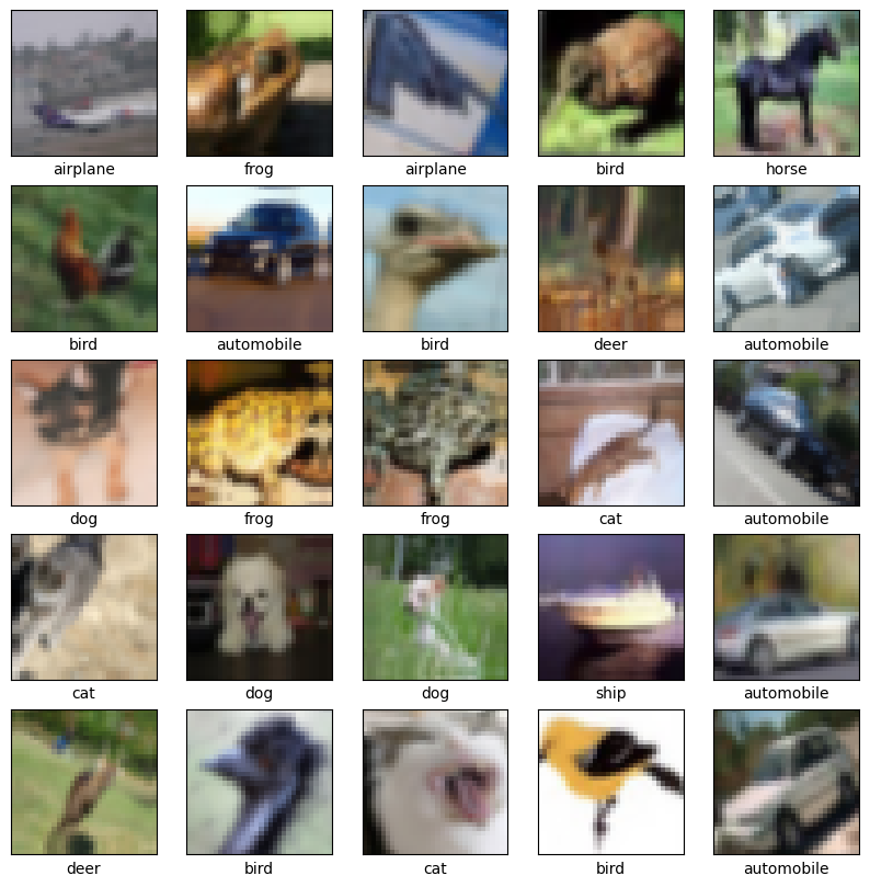
Building and Training the Model
For our improved model, we’ll adopt a more robust, VGG-inspired architecture, incorporating multiple normalization layers to stabilize training and deeper convolutional blocks to learn more intricate features.
Its core idea is to use repeating blocks of convolutional layers. Each block will consist of:
- Convolutional Layers: We use two convolutional layers back-to-back. The first one finds initial features (like edges), and the second one looks at those features to find slightly more complex patterns (like corners or textures made of those edges) before we simplify things. It’s like taking a first look, then a closer second look.
- Batch Normalization: After our convolutional layers work their magic, it steps in. It helps keep the learning process smooth and steady, like a good guide keeping everyone on track. This helps the network train faster and can also prevent it from getting too stuck on the training data (overfitting).
- Activation Function: Just like before, the
ReLUactivation helps the network make non-linear decisions, deciding which features are important enough to pass on. Note that is is put after the batch normalization, which is a pretty common practice. - Feature Condenser: After finding detailed features, it picks out the strongest signals and shrinks the information. This makes our model more efficient and helps it recognize objects even if they are slightly moved or rotated.
- Dropout: To stop our network from simply memorizing the training images (which would make it bad at recognizing new images), it randomly ignores some of the learned features during training. This forces the network to be more robust and general ways to identify objects.
By stacking these blocks, and progressively increasing the number of filters, we could build a neural network able to to perform complex visual understanding. The initial blocks might learn simple edges and colors, while deeper blocks combine these to recognize textures, parts of objects, and eventually, the objects themselves.
from tensorflow.keras import layers, Sequential

def vgg_block(filters, dropout_rate=0.15):
    return Sequential([
        layers.Conv2D(filters, (3, 3), padding='same'),
        layers.BatchNormalization(),
        layers.Activation('relu'),
        layers.Conv2D(filters, (3, 3), padding='same'),
        layers.BatchNormalization(),
        layers.Activation('relu'),
        layers.MaxPooling2D((2, 2)),
        layers.Dropout(dropout_rate),
    ])
Just as before, our model will consist of two sub-models:
- Feature Learning: Consists of multiple VGG blocks with gradual dropout, preceded by a data augmentation layer. This combination of regularization techniques makes our model less prone to overfitting.
- Classification: Essentially, it remains the same, but we may add more neurons and some batch normalization here to make it more stable.
from tensorflow.keras.utils import set_random_seed
set_random_seed(0)

feature_learning = Sequential(name='feature_learning', layers=[
    layers.Input(shape=x_train.shape[1:]),
    data_augmentation,
    vgg_block(32,  dropout_rate=0.2),
    vgg_block(64,  dropout_rate=0.3),
    vgg_block(128, dropout_rate=0.4),
    vgg_block(256, dropout_rate=0.5),
])

classification = Sequential(name = 'classification', layers=[
    layers.GlobalAveragePooling2D(),
    layers.Dense(256),
    layers.BatchNormalization(),
    layers.Activation('relu'),
    layers.Dropout(0.35),
    layers.Dense(len(class_names), activation='softmax'),
])

model = Sequential([
    feature_learning,
    classification,
])

display(model.summary(expand_nested=True))To aid our training process, we could use a combination of early stopping and learning rate scheduling callbacks. The last one will reduce the learning rate when the validation loss stops improving, helping the model to fine-tune in the later epochs.
from tensorflow.keras.callbacks import ReduceLROnPlateau, EarlyStopping
earlystop = EarlyStopping(monitor='val_loss', patience=10, restore_best_weights=True)
reduce_lr = ReduceLROnPlateau(monitor='val_loss', patience=5, factor=0.5, min_lr=0.00001)
callbacks = [reduce_lr, earlystop]
We’ll might also use the AdamW optimizer, which is an extension of the Adam optimizer that incorporates the normalization technique called weight decay, often leading to better generalization.
That’s a regularization technique that helps prevent overfitting by adding a penalty to the loss function proportional to the model’s weights. By keeping them smaller, the model tends to be simpler and less likely to fit the noise in the training data, leading to better generalization on unseen data.
from tensorflow.keras.optimizers import AdamW
optimizer = AdamW(weight_decay=0.003)
Now, let’s compile and train our final model.
from tensorflow import device
with device('/GPU'):
    model.compile(optimizer=optimizer, loss='sparse_categorical_crossentropy', metrics=['accuracy'])
    history = model.fit(x_train, y_train, epochs=100, batch_size=64, callbacks=callbacks, validation_split=0.2)
Output
Epoch 1/100
625/625 ━━━━━━━━━━━━━━━━━━━━ 45s 61ms/step - accuracy: 0.2936 - loss: 1.9783 - val_accuracy: 0.4165 - val_loss: 1.7621 - learning_rate: 0.0010
Epoch 2/100
625/625 ━━━━━━━━━━━━━━━━━━━━ 36s 58ms/step - accuracy: 0.4696 - loss: 1.4513 - val_accuracy: 0.5694 - val_loss: 1.1959 - learning_rate: 0.0010
Epoch 3/100
625/625 ━━━━━━━━━━━━━━━━━━━━ 37s 59ms/step - accuracy: 0.5458 - loss: 1.2652 - val_accuracy: 0.5249 - val_loss: 1.3685 - learning_rate: 0.0010
Epoch 4/100
625/625 ━━━━━━━━━━━━━━━━━━━━ 35s 56ms/step - accuracy: 0.5966 - loss: 1.1429 - val_accuracy: 0.5912 - val_loss: 1.1737 - learning_rate: 0.0010
Epoch 5/100
625/625 ━━━━━━━━━━━━━━━━━━━━ 35s 56ms/step - accuracy: 0.6267 - loss: 1.0608 - val_accuracy: 0.6394 - val_loss: 1.0381 - learning_rate: 0.0010
Epoch 6/100
625/625 ━━━━━━━━━━━━━━━━━━━━ 35s 56ms/step - accuracy: 0.6522 - loss: 1.0059 - val_accuracy: 0.6928 - val_loss: 0.8853 - learning_rate: 0.0010
Epoch 7/100
625/625 ━━━━━━━━━━━━━━━━━━━━ 36s 57ms/step - accuracy: 0.6657 - loss: 0.9568 - val_accuracy: 0.6801 - val_loss: 0.9543 - learning_rate: 0.0010
Epoch 8/100
625/625 ━━━━━━━━━━━━━━━━━━━━ 37s 59ms/step - accuracy: 0.6806 - loss: 0.9204 - val_accuracy: 0.6850 - val_loss: 0.9173 - learning_rate: 0.0010
Epoch 9/100
625/625 ━━━━━━━━━━━━━━━━━━━━ 38s 60ms/step - accuracy: 0.6956 - loss: 0.8873 - val_accuracy: 0.7065 - val_loss: 0.8487 - learning_rate: 0.0010
Epoch 10/100
625/625 ━━━━━━━━━━━━━━━━━━━━ 36s 57ms/step - accuracy: 0.7046 - loss: 0.8572 - val_accuracy: 0.7382 - val_loss: 0.7794 - learning_rate: 0.0010
Epoch 11/100
625/625 ━━━━━━━━━━━━━━━━━━━━ 35s 56ms/step - accuracy: 0.7136 - loss: 0.8331 - val_accuracy: 0.7188 - val_loss: 0.8157 - learning_rate: 0.0010
Epoch 12/100
625/625 ━━━━━━━━━━━━━━━━━━━━ 35s 56ms/step - accuracy: 0.7182 - loss: 0.8153 - val_accuracy: 0.6960 - val_loss: 0.8962 - learning_rate: 0.0010
Epoch 13/100
625/625 ━━━━━━━━━━━━━━━━━━━━ 35s 56ms/step - accuracy: 0.7293 - loss: 0.7935 - val_accuracy: 0.7664 - val_loss: 0.6833 - learning_rate: 0.0010
Epoch 14/100
625/625 ━━━━━━━━━━━━━━━━━━━━ 35s 56ms/step - accuracy: 0.7357 - loss: 0.7668 - val_accuracy: 0.7427 - val_loss: 0.7618 - learning_rate: 0.0010
Epoch 15/100
625/625 ━━━━━━━━━━━━━━━━━━━━ 35s 56ms/step - accuracy: 0.7433 - loss: 0.7534 - val_accuracy: 0.7636 - val_loss: 0.6724 - learning_rate: 0.0010
Epoch 16/100
625/625 ━━━━━━━━━━━━━━━━━━━━ 35s 56ms/step - accuracy: 0.7490 - loss: 0.7315 - val_accuracy: 0.7636 - val_loss: 0.7224 - learning_rate: 0.0010
Epoch 17/100
625/625 ━━━━━━━━━━━━━━━━━━━━ 35s 56ms/step - accuracy: 0.7520 - loss: 0.7193 - val_accuracy: 0.7542 - val_loss: 0.7050 - learning_rate: 0.0010
Epoch 18/100
625/625 ━━━━━━━━━━━━━━━━━━━━ 35s 56ms/step - accuracy: 0.7590 - loss: 0.7101 - val_accuracy: 0.7593 - val_loss: 0.7095 - learning_rate: 0.0010
Epoch 19/100
625/625 ━━━━━━━━━━━━━━━━━━━━ 35s 55ms/step - accuracy: 0.7591 - loss: 0.7040 - val_accuracy: 0.7548 - val_loss: 0.7294 - learning_rate: 0.0010
Epoch 20/100
625/625 ━━━━━━━━━━━━━━━━━━━━ 37s 60ms/step - accuracy: 0.7663 - loss: 0.6867 - val_accuracy: 0.7731 - val_loss: 0.6625 - learning_rate: 0.0010
Epoch 21/100
625/625 ━━━━━━━━━━━━━━━━━━━━ 37s 59ms/step - accuracy: 0.7683 - loss: 0.6746 - val_accuracy: 0.7843 - val_loss: 0.6359 - learning_rate: 0.0010
Epoch 22/100
625/625 ━━━━━━━━━━━━━━━━━━━━ 36s 57ms/step - accuracy: 0.7696 - loss: 0.6609 - val_accuracy: 0.7638 - val_loss: 0.6913 - learning_rate: 0.0010
Epoch 23/100
625/625 ━━━━━━━━━━━━━━━━━━━━ 36s 57ms/step - accuracy: 0.7750 - loss: 0.6592 - val_accuracy: 0.7588 - val_loss: 0.7069 - learning_rate: 0.0010
Epoch 24/100
625/625 ━━━━━━━━━━━━━━━━━━━━ 37s 59ms/step - accuracy: 0.7772 - loss: 0.6442 - val_accuracy: 0.7947 - val_loss: 0.6107 - learning_rate: 0.0010
Epoch 25/100
625/625 ━━━━━━━━━━━━━━━━━━━━ 36s 58ms/step - accuracy: 0.7806 - loss: 0.6390 - val_accuracy: 0.8052 - val_loss: 0.5774 - learning_rate: 0.0010
Epoch 26/100
625/625 ━━━━━━━━━━━━━━━━━━━━ 36s 58ms/step - accuracy: 0.7827 - loss: 0.6272 - val_accuracy: 0.7930 - val_loss: 0.6164 - learning_rate: 0.0010
Epoch 27/100
625/625 ━━━━━━━━━━━━━━━━━━━━ 35s 57ms/step - accuracy: 0.7886 - loss: 0.6232 - val_accuracy: 0.7851 - val_loss: 0.6220 - learning_rate: 0.0010
Epoch 28/100
625/625 ━━━━━━━━━━━━━━━━━━━━ 35s 56ms/step - accuracy: 0.7900 - loss: 0.6114 - val_accuracy: 0.7772 - val_loss: 0.6643 - learning_rate: 0.0010
Epoch 29/100
625/625 ━━━━━━━━━━━━━━━━━━━━ 35s 55ms/step - accuracy: 0.7890 - loss: 0.6109 - val_accuracy: 0.8011 - val_loss: 0.5880 - learning_rate: 0.0010
Epoch 30/100
625/625 ━━━━━━━━━━━━━━━━━━━━ 35s 56ms/step - accuracy: 0.7980 - loss: 0.5924 - val_accuracy: 0.7708 - val_loss: 0.6744 - learning_rate: 0.0010
Epoch 31/100
625/625 ━━━━━━━━━━━━━━━━━━━━ 35s 55ms/step - accuracy: 0.8021 - loss: 0.5732 - val_accuracy: 0.8178 - val_loss: 0.5429 - learning_rate: 5.0000e-04
Epoch 32/100
625/625 ━━━━━━━━━━━━━━━━━━━━ 34s 55ms/step - accuracy: 0.8152 - loss: 0.5459 - val_accuracy: 0.8329 - val_loss: 0.4903 - learning_rate: 5.0000e-04
Epoch 33/100
625/625 ━━━━━━━━━━━━━━━━━━━━ 35s 55ms/step - accuracy: 0.8167 - loss: 0.5371 - val_accuracy: 0.8034 - val_loss: 0.5771 - learning_rate: 5.0000e-04
Epoch 34/100
625/625 ━━━━━━━━━━━━━━━━━━━━ 35s 55ms/step - accuracy: 0.8187 - loss: 0.5374 - val_accuracy: 0.8194 - val_loss: 0.5449 - learning_rate: 5.0000e-04
Epoch 35/100
625/625 ━━━━━━━━━━━━━━━━━━━━ 35s 56ms/step - accuracy: 0.8197 - loss: 0.5238 - val_accuracy: 0.8261 - val_loss: 0.5149 - learning_rate: 5.0000e-04
Epoch 36/100
625/625 ━━━━━━━━━━━━━━━━━━━━ 36s 57ms/step - accuracy: 0.8208 - loss: 0.5265 - val_accuracy: 0.8290 - val_loss: 0.4924 - learning_rate: 5.0000e-04
Epoch 37/100
625/625 ━━━━━━━━━━━━━━━━━━━━ 37s 60ms/step - accuracy: 0.8218 - loss: 0.5137 - val_accuracy: 0.8289 - val_loss: 0.5170 - learning_rate: 5.0000e-04
Epoch 38/100
625/625 ━━━━━━━━━━━━━━━━━━━━ 36s 58ms/step - accuracy: 0.8256 - loss: 0.5018 - val_accuracy: 0.8447 - val_loss: 0.4672 - learning_rate: 2.5000e-04
Epoch 39/100
625/625 ━━━━━━━━━━━━━━━━━━━━ 36s 58ms/step - accuracy: 0.8282 - loss: 0.4982 - val_accuracy: 0.8486 - val_loss: 0.4536 - learning_rate: 2.5000e-04
Epoch 40/100
625/625 ━━━━━━━━━━━━━━━━━━━━ 36s 58ms/step - accuracy: 0.8339 - loss: 0.4837 - val_accuracy: 0.8502 - val_loss: 0.4513 - learning_rate: 2.5000e-04
Epoch 41/100
625/625 ━━━━━━━━━━━━━━━━━━━━ 35s 57ms/step - accuracy: 0.8340 - loss: 0.4797 - val_accuracy: 0.8466 - val_loss: 0.4674 - learning_rate: 2.5000e-04
Epoch 42/100
625/625 ━━━━━━━━━━━━━━━━━━━━ 37s 59ms/step - accuracy: 0.8357 - loss: 0.4785 - val_accuracy: 0.8455 - val_loss: 0.4614 - learning_rate: 2.5000e-04
Epoch 43/100
625/625 ━━━━━━━━━━━━━━━━━━━━ 36s 58ms/step - accuracy: 0.8362 - loss: 0.4763 - val_accuracy: 0.8498 - val_loss: 0.4465 - learning_rate: 2.5000e-04
Epoch 44/100
625/625 ━━━━━━━━━━━━━━━━━━━━ 36s 57ms/step - accuracy: 0.8386 - loss: 0.4652 - val_accuracy: 0.8518 - val_loss: 0.4417 - learning_rate: 2.5000e-04
Epoch 45/100
625/625 ━━━━━━━━━━━━━━━━━━━━ 35s 56ms/step - accuracy: 0.8381 - loss: 0.4695 - val_accuracy: 0.8454 - val_loss: 0.4630 - learning_rate: 2.5000e-04
Epoch 46/100
625/625 ━━━━━━━━━━━━━━━━━━━━ 35s 56ms/step - accuracy: 0.8364 - loss: 0.4666 - val_accuracy: 0.8498 - val_loss: 0.4485 - learning_rate: 2.5000e-04
Epoch 47/100
625/625 ━━━━━━━━━━━━━━━━━━━━ 35s 56ms/step - accuracy: 0.8388 - loss: 0.4654 - val_accuracy: 0.8515 - val_loss: 0.4420 - learning_rate: 2.5000e-04
Epoch 48/100
625/625 ━━━━━━━━━━━━━━━━━━━━ 36s 57ms/step - accuracy: 0.8416 - loss: 0.4588 - val_accuracy: 0.8495 - val_loss: 0.4452 - learning_rate: 2.5000e-04
Epoch 49/100
625/625 ━━━━━━━━━━━━━━━━━━━━ 35s 56ms/step - accuracy: 0.8414 - loss: 0.4556 - val_accuracy: 0.8519 - val_loss: 0.4429 - learning_rate: 2.5000e-04
Epoch 50/100
625/625 ━━━━━━━━━━━━━━━━━━━━ 35s 56ms/step - accuracy: 0.8419 - loss: 0.4567 - val_accuracy: 0.8548 - val_loss: 0.4314 - learning_rate: 1.2500e-04
Epoch 51/100
625/625 ━━━━━━━━━━━━━━━━━━━━ 35s 55ms/step - accuracy: 0.8510 - loss: 0.4395 - val_accuracy: 0.8551 - val_loss: 0.4362 - learning_rate: 1.2500e-04
Epoch 52/100
625/625 ━━━━━━━━━━━━━━━━━━━━ 35s 56ms/step - accuracy: 0.8473 - loss: 0.4436 - val_accuracy: 0.8571 - val_loss: 0.4261 - learning_rate: 1.2500e-04
Epoch 53/100
625/625 ━━━━━━━━━━━━━━━━━━━━ 34s 55ms/step - accuracy: 0.8469 - loss: 0.4424 - val_accuracy: 0.8583 - val_loss: 0.4221 - learning_rate: 1.2500e-04
Epoch 54/100
625/625 ━━━━━━━━━━━━━━━━━━━━ 35s 56ms/step - accuracy: 0.8480 - loss: 0.4363 - val_accuracy: 0.8593 - val_loss: 0.4212 - learning_rate: 1.2500e-04
Epoch 55/100
625/625 ━━━━━━━━━━━━━━━━━━━━ 35s 55ms/step - accuracy: 0.8475 - loss: 0.4336 - val_accuracy: 0.8599 - val_loss: 0.4178 - learning_rate: 1.2500e-04
Epoch 56/100
625/625 ━━━━━━━━━━━━━━━━━━━━ 37s 59ms/step - accuracy: 0.8469 - loss: 0.4418 - val_accuracy: 0.8590 - val_loss: 0.4265 - learning_rate: 1.2500e-04
Epoch 57/100
625/625 ━━━━━━━━━━━━━━━━━━━━ 35s 56ms/step - accuracy: 0.8474 - loss: 0.4387 - val_accuracy: 0.8514 - val_loss: 0.4412 - learning_rate: 1.2500e-04
Epoch 58/100
625/625 ━━━━━━━━━━━━━━━━━━━━ 36s 58ms/step - accuracy: 0.8508 - loss: 0.4301 - val_accuracy: 0.8586 - val_loss: 0.4303 - learning_rate: 1.2500e-04
Epoch 59/100
625/625 ━━━━━━━━━━━━━━━━━━━━ 35s 56ms/step - accuracy: 0.8477 - loss: 0.4354 - val_accuracy: 0.8648 - val_loss: 0.4107 - learning_rate: 1.2500e-04
Epoch 60/100
625/625 ━━━━━━━━━━━━━━━━━━━━ 37s 60ms/step - accuracy: 0.8467 - loss: 0.4346 - val_accuracy: 0.8559 - val_loss: 0.4395 - learning_rate: 1.2500e-04
Epoch 61/100
625/625 ━━━━━━━━━━━━━━━━━━━━ 36s 57ms/step - accuracy: 0.8508 - loss: 0.4274 - val_accuracy: 0.8607 - val_loss: 0.4222 - learning_rate: 1.2500e-04
Epoch 62/100
625/625 ━━━━━━━━━━━━━━━━━━━━ 39s 62ms/step - accuracy: 0.8491 - loss: 0.4294 - val_accuracy: 0.8565 - val_loss: 0.4276 - learning_rate: 1.2500e-04
Epoch 63/100
625/625 ━━━━━━━━━━━━━━━━━━━━ 36s 58ms/step - accuracy: 0.8496 - loss: 0.4331 - val_accuracy: 0.8589 - val_loss: 0.4231 - learning_rate: 1.2500e-04
Epoch 64/100
625/625 ━━━━━━━━━━━━━━━━━━━━ 37s 59ms/step - accuracy: 0.8509 - loss: 0.4287 - val_accuracy: 0.8589 - val_loss: 0.4207 - learning_rate: 1.2500e-04
Epoch 65/100
625/625 ━━━━━━━━━━━━━━━━━━━━ 37s 59ms/step - accuracy: 0.8521 - loss: 0.4263 - val_accuracy: 0.8603 - val_loss: 0.4176 - learning_rate: 6.2500e-05
Epoch 66/100
625/625 ━━━━━━━━━━━━━━━━━━━━ 37s 59ms/step - accuracy: 0.8552 - loss: 0.4208 - val_accuracy: 0.8659 - val_loss: 0.4019 - learning_rate: 6.2500e-05
Epoch 67/100
625/625 ━━━━━━━━━━━━━━━━━━━━ 36s 58ms/step - accuracy: 0.8520 - loss: 0.4234 - val_accuracy: 0.8617 - val_loss: 0.4158 - learning_rate: 6.2500e-05
Epoch 68/100
625/625 ━━━━━━━━━━━━━━━━━━━━ 35s 56ms/step - accuracy: 0.8548 - loss: 0.4156 - val_accuracy: 0.8624 - val_loss: 0.4166 - learning_rate: 6.2500e-05
Epoch 69/100
625/625 ━━━━━━━━━━━━━━━━━━━━ 36s 57ms/step - accuracy: 0.8539 - loss: 0.4220 - val_accuracy: 0.8634 - val_loss: 0.4092 - learning_rate: 6.2500e-05
Epoch 70/100
625/625 ━━━━━━━━━━━━━━━━━━━━ 37s 59ms/step - accuracy: 0.8587 - loss: 0.4106 - val_accuracy: 0.8619 - val_loss: 0.4128 - learning_rate: 6.2500e-05
Epoch 71/100
625/625 ━━━━━━━━━━━━━━━━━━━━ 38s 60ms/step - accuracy: 0.8535 - loss: 0.4201 - val_accuracy: 0.8665 - val_loss: 0.4050 - learning_rate: 6.2500e-05
Epoch 72/100
625/625 ━━━━━━━━━━━━━━━━━━━━ 40s 64ms/step - accuracy: 0.8549 - loss: 0.4186 - val_accuracy: 0.8641 - val_loss: 0.4085 - learning_rate: 3.1250e-05
Epoch 73/100
625/625 ━━━━━━━━━━━━━━━━━━━━ 38s 61ms/step - accuracy: 0.8578 - loss: 0.4159 - val_accuracy: 0.8631 - val_loss: 0.4113 - learning_rate: 3.1250e-05
Epoch 74/100
625/625 ━━━━━━━━━━━━━━━━━━━━ 37s 60ms/step - accuracy: 0.8573 - loss: 0.4109 - val_accuracy: 0.8647 - val_loss: 0.4061 - learning_rate: 3.1250e-05
Epoch 75/100
625/625 ━━━━━━━━━━━━━━━━━━━━ 35s 57ms/step - accuracy: 0.8567 - loss: 0.4157 - val_accuracy: 0.8642 - val_loss: 0.4049 - learning_rate: 3.1250e-05
Epoch 76/100
625/625 ━━━━━━━━━━━━━━━━━━━━ 37s 59ms/step - accuracy: 0.8559 - loss: 0.4149 - val_accuracy: 0.8634 - val_loss: 0.4139 - learning_rate: 3.1250e-05
import matplotlib.pyplot as plt
plt.figure(figsize=(4.5, 3))
plt.plot(history.history['accuracy'], label='train')
plt.plot(history.history['val_accuracy'], label='validation')
plt.ylabel('accuracy')
plt.xlabel('epoch')
plt.legend(loc='lower right')
plt.show()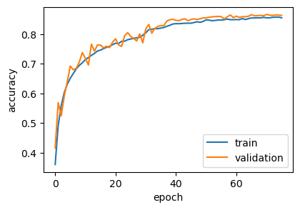
Result
from sklearn.metrics import classification_report
with device('/GPU'):
    y_pred_values = model.predict(x_test, verbose=False)
    y_pred_labels = np.argmax(y_pred_values, axis=1)
    print(classification_report(y_test, y_pred_labels, target_names=class_names))
precision recall f1-score support
airplane 0.88 0.87 0.87 1000
automobile 0.90 0.94 0.92 1000
bird 0.88 0.77 0.82 1000
cat 0.82 0.68 0.74 1000
deer 0.83 0.83 0.83 1000
dog 0.85 0.76 0.80 1000
frog 0.80 0.95 0.87 1000
horse 0.85 0.93 0.89 1000
ship 0.93 0.91 0.92 1000
truck 0.84 0.94 0.89 1000
accuracy 0.86 10000
macro avg 0.86 0.86 0.86 10000
weighted avg 0.86 0.86 0.86 10000
from sklearn.metrics import ConfusionMatrixDisplay
import matplotlib.pyplot as plt
_, ax = plt.subplots(1, 1, figsize=(3.5, 3.5))
ConfusionMatrixDisplay.from_predictions(
    y_test,
    y_pred_labels,
    display_labels=class_names,
    normalize='pred',
    xticks_rotation='vertical',
    include_values=False,
    ax=ax
)
<sklearn.metrics._plot.confusion_matrix.ConfusionMatrixDisplay at 0x31f5a43a0>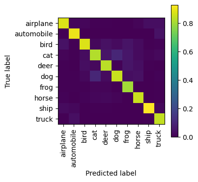
Conclusion
By systematically incorporating data augmentation, architectural changes, and training callbacks, we have substantially boosted our model’s performance. The leap to a much more compelling 86% accuracy on the CIFAR-10 test set clearly demonstrates the power of these combined techniques.
More importantly, these improvements weren’t just about chasing a higher accuracy figure - they were crucial in addressing the overfitting observed previously. The model now generalizes better to unseen data, making it much more reliable.
While this tuned model shows significant progress, future improvements could involve experimenting with even deeper or wider networks, attention mechanisms, or leveraging transfer learning for even greater accuracy.