Recurrent Neural Networks

In our previous MLP experiment, we saw that a neural network could extract more from averaged word embeddings than a simple Logistic Regression. However, averaging throws away crucial information - the order of words in a sentence.

This time, we are going to dive deeper into recurrent neural networks. They are specifically designed to process sequences, remembering context and understanding how word order contributes to meaning. Let’s see if harnessing this sequential power can push our accuracy even further.

Data Preparation¶

In our previous notebook, we simply tokenized text and then immediately squashed it into the averaged word vectors. Our new recurrent pipeline needs to be a bit more complicated.

This time, we would simply tokenize our sentences first - without trying to vectorize them. We might limit the vocabulary, making it more robust and accurate representation of frequently occurring words by filtering out rare or noisy terms.

Next, we need to pad our sequences. Most neural networks require input sequences to be of a uniform length. Since our sentences naturally vary, we need to bring them to the same length.

This involves either truncating longer sequences or adding special tokens (usually zeros) to shorter sequences until they all reach a predetermined maximum length. Let’s do a small research to determine how long our sequences usually are.

Taking the top quartile length seems to be a reasonable choice here.

Embedding Layer¶

Finally, we need to transform these padded sequences into some meaningful representation that captures their semantic relationships. That’s where the embedding layer comes in. To build it, we may utilize our existing pre-trained model.

Think of it as some sort of a lookup table - for each token in our sequence, the embedding layer looks up its corresponding dense vector. This helps our neural network to capture not some random indexes, but the semantic meaning of words.

Building and Training the Model¶

Here comes the most interesting part.

With our text now represented as sequences of dense semantic vectors (thanks to the embedding layer), we can introduce the star of this experiment - the Gated Recurrent Unit (GRU) layer. Unlike a simple dense layer that processes all its inputs at once, a GRU layer processes each vector in our sequence one at a time. Internally, each GRU unit contains two gates – an update gate, and a reset gate.

These gates learn to control the flow of information, deciding what to remember from previous steps, what to discard, and what new information from the current word’s vector is important enough to update its hidden memory, allowing it to capture context and dependencies across the entire sequence.

We may also make the recurrent layer bidirectional, wrapping it in a special helper function - this will allow the network to capture information from both past and future time steps, leading to a more comprehensive understanding of the sequence.

Before we start the training, we might tweak a few more things. Changing the optimizer learning rate may be a good idea - the default one might be too high when using pre-trained embeddings.

We might also use our early stopping callback again.

Finally, let’s compile and train our final model. This time we might start using the GPU - our model is finally complex enough to leverage the parallelism it offers to speed up the training process.

Result¶

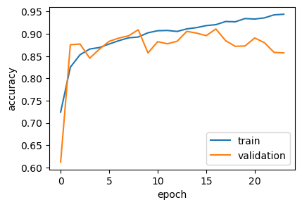
Conclusion¶

We achieved a final accuracy of 90%, finally reaching the original TF-IDF linear model level. The learning curve is still a bit wonky, but it looks much, much healthier now.

This proves the value of sequence-aware models over simple embedding averaging for this kind of task, performing competitively with the heavily optimized linear approach. Further improvements would require exploring more advanced architectures like transformers.