Previously, we tried using word embeddings to improve our sentiment classification, but instead of a better score, we got a worse result. That happened because our existing architecture (logistic regression) was unfit for a new vectorization (seemingly much better) approach. But what if we change the architecture itself?
That gives us a nice opportunity to try a different paradigm called deep learning - a branch of machine learning and artificial intelligence that uses artificial neural networks to process data and learn patterns. These networks, inspired by the structure of the human brain, are built with multiple layers of interconnected neurons that allow them to identify complex relationships and make predictions.
Data Preparation
from datasets import load_dataset
import numpy as np

train, test = load_dataset('stanfordnlp/imdb', split=['train', 'test'])
class_names = train.features['label'].names

x_train = np.array(train['text'])
y_train = np.array(train['label'])
x_test = np.array(test['text'])
y_test = np.array(test['label'])
Our vectorization routine also remains exactly the same. We are doing this to see how the change in approach affects the final result without touching any preparational routines.
from gensim.models import KeyedVectors
from gensim.utils import simple_preprocess
from huggingface_hub import snapshot_download
from os import path

model_path = path.join(snapshot_download('fse/word2vec-google-news-300'), 'word2vec-google-news-300.model')
wv = KeyedVectors.load(model_path)

def vectorize(text):
    tokens = simple_preprocess(text.lower(), deacc=True)
    token_vectors = [wv.get_vector(x) for x in tokens if x in wv]
    if token_vectors:
        return np.mean(token_vectors, axis=0)
    else:
        return np.zeros(wv.vector_size)
Output
We need to transform our data before passing it to the model. That happens because neural networks are generally unable to process textual information directly - instead, we need to encode our data, turning it into some kind of mathematical representation.
x_train = np.array([vectorize(seq) for seq in x_train])
x_test = np.array([vectorize(seq) for seq in x_test])
Building and Training the Model
Now, let’s design our model structure. This time, we will use a thing called multilayer perceptron. As its name states, it is a neural network that consists of multiple layers of neurons - allowing one to learn complex, non-linear relationships in data (unlike linear regression classifier).
For this task, we will use three types of layers:
- Input: Transforms our source data and passes it next.
- Dense: Layer of densely connected neurons (each neuron is connected to all other neurons of the neighboring layers).
- Dropuput: Special layer that helps against overfitting by randomly disabling parts of the previous layer during the training process.
We may experiment with number of hidden layers and dropout rates - those are, in fact, hyperplanar parameters that may be tuned. Stack more layers meme, you know.
from tensorflow.keras.utils import set_random_seed
from tensorflow.keras import layers, Sequential

num_classes = len(class_names)
set_random_seed(0)

model = Sequential([
    layers.Input(shape=(wv.vector_size,)),
    layers.Dense(256, activation='relu'),
    layers.Dropout(0.4),
    layers.Dense(256, activation='relu'),
    layers.Dropout(0.3),
    layers.Dense(256, activation='relu'),
    layers.Dropout(0.2),
    layers.Dense(num_classes, activation='softmax')
])

display(model.summary())To aid our training process, we could use an early stopping callback. It stops the training process if the validation loss doesn’t improve for a set number of epochs, also restoring the best possible weights.
from tensorflow.keras.callbacks import EarlyStopping
earlystop = EarlyStopping(monitor='val_loss', patience=10, restore_best_weights=True)
We can compile and train our model now. Sticking to the CPU may be a good idea for now - using GPU for such a small model may actually slow down the training process due to a huge data transfer overhead.
from tensorflow import device
with device('/CPU'):
    model.compile(optimizer='adam', loss='sparse_categorical_crossentropy', metrics=['accuracy'])
    history = model.fit(x_train, y_train, epochs=50, batch_size=64, callbacks=[earlystop], validation_split=0.2)
Output
Epoch 1/50
313/313 ━━━━━━━━━━━━━━━━━━━━ 2s 4ms/step - accuracy: 0.7208 - loss: 0.5272 - val_accuracy: 0.6092 - val_loss: 0.8005
Epoch 2/50
313/313 ━━━━━━━━━━━━━━━━━━━━ 1s 4ms/step - accuracy: 0.8394 - loss: 0.3675 - val_accuracy: 0.5910 - val_loss: 0.8200
Epoch 3/50
313/313 ━━━━━━━━━━━━━━━━━━━━ 1s 4ms/step - accuracy: 0.8457 - loss: 0.3535 - val_accuracy: 0.7012 - val_loss: 0.6369
Epoch 4/50
313/313 ━━━━━━━━━━━━━━━━━━━━ 1s 4ms/step - accuracy: 0.8533 - loss: 0.3419 - val_accuracy: 0.7188 - val_loss: 0.6045
Epoch 5/50
313/313 ━━━━━━━━━━━━━━━━━━━━ 1s 4ms/step - accuracy: 0.8581 - loss: 0.3360 - val_accuracy: 0.7254 - val_loss: 0.6127
Epoch 6/50
313/313 ━━━━━━━━━━━━━━━━━━━━ 1s 4ms/step - accuracy: 0.8545 - loss: 0.3373 - val_accuracy: 0.7362 - val_loss: 0.5887
Epoch 7/50
313/313 ━━━━━━━━━━━━━━━━━━━━ 1s 4ms/step - accuracy: 0.8609 - loss: 0.3271 - val_accuracy: 0.7150 - val_loss: 0.6063
Epoch 8/50
313/313 ━━━━━━━━━━━━━━━━━━━━ 1s 4ms/step - accuracy: 0.8632 - loss: 0.3212 - val_accuracy: 0.7416 - val_loss: 0.5711
Epoch 9/50
313/313 ━━━━━━━━━━━━━━━━━━━━ 1s 5ms/step - accuracy: 0.8608 - loss: 0.3264 - val_accuracy: 0.7438 - val_loss: 0.5444
Epoch 10/50
313/313 ━━━━━━━━━━━━━━━━━━━━ 1s 4ms/step - accuracy: 0.8628 - loss: 0.3227 - val_accuracy: 0.7446 - val_loss: 0.5518
Epoch 11/50
313/313 ━━━━━━━━━━━━━━━━━━━━ 1s 4ms/step - accuracy: 0.8648 - loss: 0.3197 - val_accuracy: 0.7716 - val_loss: 0.5086
Epoch 12/50
313/313 ━━━━━━━━━━━━━━━━━━━━ 1s 4ms/step - accuracy: 0.8649 - loss: 0.3167 - val_accuracy: 0.7790 - val_loss: 0.4943
Epoch 13/50
313/313 ━━━━━━━━━━━━━━━━━━━━ 1s 4ms/step - accuracy: 0.8687 - loss: 0.3149 - val_accuracy: 0.7340 - val_loss: 0.5688
Epoch 14/50
313/313 ━━━━━━━━━━━━━━━━━━━━ 1s 4ms/step - accuracy: 0.8650 - loss: 0.3155 - val_accuracy: 0.7840 - val_loss: 0.4723
Epoch 15/50
313/313 ━━━━━━━━━━━━━━━━━━━━ 1s 5ms/step - accuracy: 0.8679 - loss: 0.3099 - val_accuracy: 0.7924 - val_loss: 0.4441
Epoch 16/50
313/313 ━━━━━━━━━━━━━━━━━━━━ 1s 4ms/step - accuracy: 0.8681 - loss: 0.3124 - val_accuracy: 0.7322 - val_loss: 0.5487
Epoch 17/50
313/313 ━━━━━━━━━━━━━━━━━━━━ 1s 4ms/step - accuracy: 0.8690 - loss: 0.3077 - val_accuracy: 0.7694 - val_loss: 0.4744
Epoch 18/50
313/313 ━━━━━━━━━━━━━━━━━━━━ 1s 4ms/step - accuracy: 0.8680 - loss: 0.3102 - val_accuracy: 0.7946 - val_loss: 0.4560
Epoch 19/50
313/313 ━━━━━━━━━━━━━━━━━━━━ 1s 4ms/step - accuracy: 0.8684 - loss: 0.3081 - val_accuracy: 0.8142 - val_loss: 0.4520
Epoch 20/50
313/313 ━━━━━━━━━━━━━━━━━━━━ 1s 5ms/step - accuracy: 0.8693 - loss: 0.3047 - val_accuracy: 0.7832 - val_loss: 0.4689
Epoch 21/50
313/313 ━━━━━━━━━━━━━━━━━━━━ 1s 4ms/step - accuracy: 0.8751 - loss: 0.3061 - val_accuracy: 0.7548 - val_loss: 0.5439
Epoch 22/50
313/313 ━━━━━━━━━━━━━━━━━━━━ 1s 4ms/step - accuracy: 0.8702 - loss: 0.3072 - val_accuracy: 0.7696 - val_loss: 0.5065
Epoch 23/50
313/313 ━━━━━━━━━━━━━━━━━━━━ 1s 4ms/step - accuracy: 0.8742 - loss: 0.2968 - val_accuracy: 0.7706 - val_loss: 0.5032
Epoch 24/50
313/313 ━━━━━━━━━━━━━━━━━━━━ 1s 4ms/step - accuracy: 0.8734 - loss: 0.2981 - val_accuracy: 0.8344 - val_loss: 0.3897
Epoch 25/50
313/313 ━━━━━━━━━━━━━━━━━━━━ 1s 4ms/step - accuracy: 0.8736 - loss: 0.2978 - val_accuracy: 0.7834 - val_loss: 0.4955
Epoch 26/50
313/313 ━━━━━━━━━━━━━━━━━━━━ 1s 4ms/step - accuracy: 0.8758 - loss: 0.2979 - val_accuracy: 0.8112 - val_loss: 0.4303
Epoch 27/50
313/313 ━━━━━━━━━━━━━━━━━━━━ 3s 10ms/step - accuracy: 0.8763 - loss: 0.2970 - val_accuracy: 0.7578 - val_loss: 0.5271
Epoch 28/50
313/313 ━━━━━━━━━━━━━━━━━━━━ 2s 5ms/step - accuracy: 0.8780 - loss: 0.2940 - val_accuracy: 0.7862 - val_loss: 0.4686
Epoch 29/50
313/313 ━━━━━━━━━━━━━━━━━━━━ 2s 6ms/step - accuracy: 0.8733 - loss: 0.2961 - val_accuracy: 0.7462 - val_loss: 0.5722
Epoch 30/50
313/313 ━━━━━━━━━━━━━━━━━━━━ 1s 4ms/step - accuracy: 0.8753 - loss: 0.2944 - val_accuracy: 0.7798 - val_loss: 0.5048
Epoch 31/50
313/313 ━━━━━━━━━━━━━━━━━━━━ 1s 4ms/step - accuracy: 0.8767 - loss: 0.2927 - val_accuracy: 0.8176 - val_loss: 0.4332
Epoch 32/50
313/313 ━━━━━━━━━━━━━━━━━━━━ 1s 4ms/step - accuracy: 0.8784 - loss: 0.2917 - val_accuracy: 0.8220 - val_loss: 0.4400
Epoch 33/50
313/313 ━━━━━━━━━━━━━━━━━━━━ 1s 4ms/step - accuracy: 0.8794 - loss: 0.2885 - val_accuracy: 0.7840 - val_loss: 0.5253
Epoch 34/50
313/313 ━━━━━━━━━━━━━━━━━━━━ 1s 4ms/step - accuracy: 0.8785 - loss: 0.2876 - val_accuracy: 0.7640 - val_loss: 0.5426
Result
from sklearn.metrics import classification_report
with device('/CPU'):
    y_pred_values = model.predict(x_test, verbose=False)
    y_pred_labels = np.argmax(y_pred_values, axis=1)
    print(classification_report(y_test, y_pred_labels, target_names=class_names))
precision recall f1-score support
neg 0.85 0.88 0.86 12500
pos 0.87 0.84 0.86 12500
accuracy 0.86 25000
macro avg 0.86 0.86 0.86 25000
weighted avg 0.86 0.86 0.86 25000
Let’s take a look at the training history - it may tell us a lot.
import matplotlib.pyplot as plt
plt.figure(figsize=(4.5, 3))
plt.plot(history.history['accuracy'], label='train')
plt.plot(history.history['val_accuracy'], label='validation')
plt.ylabel('accuracy')
plt.xlabel('epoch')
plt.legend(loc='lower right')
plt.show()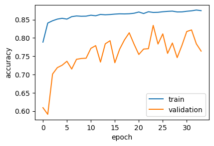
We can observe that the training accuracy steadily increases, indicating the model is continuously learning from the training data. However, the validation accuracy shows a different trend - it rises initially but then begins to plateau around epoch 15-20.
The gap between the training and validation accuracy in later epochs is a classic sign of overfitting, where the model becomes too specialized in the training examples, essentially memorizing them. To mitigate this, we might need more training data, or a better model architecture.
Conclusion
This experiment yielded an 86% accuracy. While this is the same result as the previous linear model, it demonstrates an entirely different approach to machine learning. The addition of hidden layers and dropout underscores the “stack more layers” principle - at least to a point.
Nevertheless, it still trails our original TF-IDF model. This suggests that to fully leverage word embeddings, we might need an architecture capable of processing sequences to leverage the semantic richness of word embeddings.